Next time you are stuck at traffic lights you will think of neutrino beams

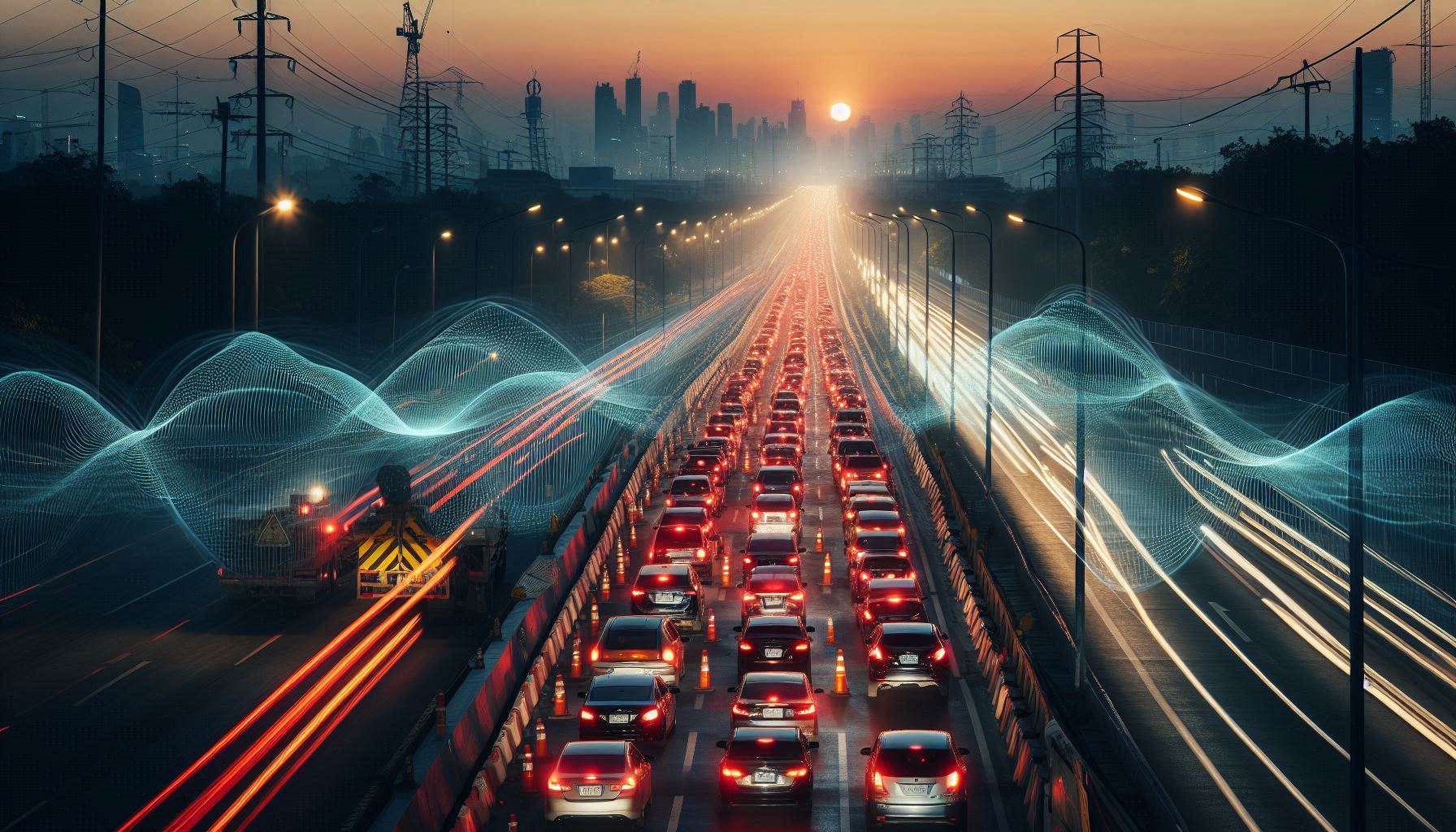
You have been sitting still for two minutes.

The opposite lane gets another green. A fresh burst of cars streams past. Your foot hovers above the brake, ready for the moment your own lane finally wakes up.

You cannot see the lights. No line of sight.

And yet you already have a sense of:

• how long the cycle is,
• when your lane will release,
• roughly how far away the junction must be.

That feeling is not superstition. It is inference.

What your brain is doing in a queue is extremely close to what experimental physicists do with neutrino beams: reconstruct a hidden controller from nothing but timing, bursts, and delayed response.

1) The only clues you have

In a blocked lane you can observe:

• bursts (cars stream, then silence),
• gaps (silence between bursts),
• delay (time from “release begins at the head” to “I begin to move”).

From those you can infer:

• the signal period $T$,
• the green splits,
• the queue length ahead of you,
• and therefore the distance to an unseen junction.

This is a textbook inverse problem: you see outputs, not the mechanism.

2) A minimal model

Assume a two-way temporary light:

• Lane A (opposite direction) green for $g_A$​
• all-red safety gap $\Delta$
• Lane B (your direction) green for $g_B$
• all-red safety gap $\Delta$

Two empirical constants (good enough for order-of-magnitude inference):

• saturation headway (once moving): about 2 s per car
• jam spacing: about 6 m per car (car + compressed gap)

In a stationary queue, the “release” propagates backwards: each car begins moving a bit after the one ahead. Modelling that as roughly “a couple of seconds per car” is crude but works surprisingly well near the front.

3) Fully worked example: solving an invisible junction

You are in Lane B. You time the opposite lane:

• Cars stream for 22 s → estimate $g_A \approx 22$ s
• Then nothing for 36 s → estimate $g_B + 2\Delta \approx 36$ s

So the total period is:$$T \approx 22 + 36 = 58\ \text{s}$$

Now infer your position in the queue.

You track your own release relative to the opposite burst:

• $t = 0$: opposing flow begins
• $t \approx 22$: opposing flow ends
• (gap, then your lane’s release begins at the junction)
• $t \approx 40$: you begin to move

Suppose you estimate your lane’s release begins at the head around $t \approx 25$ (opposing ends at 22, then a short all-red, then your green). Then the propagation delay from head to you is:

$$40 – 25 = 15\ \text{s}$$

With about 2 s per car:$$15 \approx 2N \Rightarrow N \approx 7.5$$

Distance to the light:$$D \approx 7.5 \times 6\ \text{m} \approx 45\ \text{m}$$

You just estimated distance to a junction you cannot see—within a few car lengths—using timing alone.

4) Long queues: multiple greens before you move

If you are far enough back that your lane does not clear on the next green, you extend the same logic.

If your green is $g_B$​, and cars discharge about one every 2 seconds, then cars served per green is roughly:

$$G \approx \frac{g_B}{2}$$

If you sit through two full greens without moving, that suggests you are at least $2G$ cars back from the release front (plus whatever is left over).

On the third green, if you begin moving $x$x seconds after release begins, then you are about $x/2$x/2 cars into that release.

5) Where the method breaks

Far enough upstream, you stop seeing the light’s structure and start seeing traffic as a wave medium:

• stop–go waves propagate backwards,
• gaps compress and expand,
• side roads inject vehicles,
• signals may be adaptive (no fixed $T$).

In that regime, your motion reflects local traffic dynamics more than the junction controller. The “information” about the light decays with distance.

That breakdown is itself the physics.

6) Stretch the road to 500 km: neutrino beams

In many neutrino experiments:

• you cannot see the beam,
• most particles are never detected,
• the source is hundreds of kilometres away,
• you only get sparse bursts of detector events.

Physicists infer:

• beam spill timing and duration,
• periodicity and drift,
• intensity,
• and parameters that reshape the burst pattern.

Cars → neutrino interactions
Bursts → beam spills
Silence → beam-off cycle
Delay → synchronization / propagation / phase effects
Noise cars → cosmic-ray / radioactive / instrumentation backgrounds

Hidden controller → burst pattern → distant observer reconstructs mechanism.

7) Background events

A random car appears mid-silence from a farm track.

It does not match:

• timing,
• clustering,
• spacing.

You treat it as noise.

That is exactly what neutrino analyses do: classify out-of-pattern events as background.

8) The payoff

Time the opposing burst. Time the gap. Time the delay to your own motion.

Do the inference.

When you finally roll past the lights, check.

You will often be within a car length or two.

Traffic jams are boring. The inverse problem underneath them is not.

https://thinkinginstructure.substack.com/p/next-time-you-are-stuck-at-traffic